Concepts of Community Analysis

How can we examine microbial communities?

Let’s switch datasets and look at: The American Gut Project (AGP)

American Gut Project (AGP) logo. Source: http://humanfoodproject.com/americangut/

Why?

• Clustering features, creating a phylogeny, and assigning taxonomy are the most computationally intensive

  • We used very small and sparse data
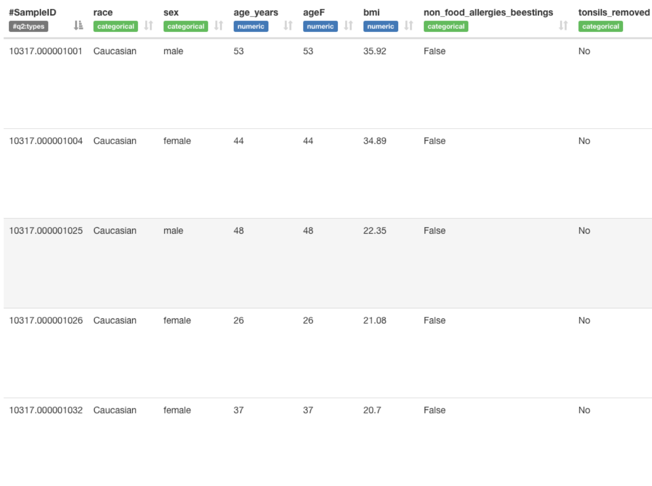
  • This subset of the AGP has 1,375 individuals
  • There are 5,590 features (bacteria) and ~200 metadata measurements

• You may get processed data from a colaborator / website already as a table, phylogeny…

  • Need to know how to import at any stage of the project
  • QIIME2 Importing Tutorial

  • There are far more options than even they show

    • Check the docs: qiime tools import –help
    • There are many types of data: qiime tools import –show-importable-types
    • For each type there are many subformats: qiime tools import –show-importable-formats

Importing the AGP

1. Look at the files in the american_gut folder
2. Import the biom table
3. Import the bacterial phylogeny
4. Look at the available metadata

# See the files we will work with
ls -lsh american_gut

# Import the biom count table of features by samples
qiime tools import \
  --input-path  american_gut/1_0_biom.biom \
  --type 'FeatureTable[Frequency]' \
  --input-format BIOMV100Format \
  --output-path american_gut/1_1_biom.qza

# Import the bacterial 16S phylogeny
qiime tools import \
  --input-path american_gut/1_0_tree.tre \
  --output-path american_gut/1_1_tree.qza \
  --type 'Phylogeny[Rooted]'

# Import the bacterial taxonomy
qiime tools import \
   --input-path american_gut/1_0_tax.tsv \
   --output-path american_gut/1_1_tax.qza \
   --type FeatureData[Taxonomy] \
   --input-format HeaderlessTSVTaxonomyFormat

# Create a visual of the metadata (map.txt)
qiime metadata tabulate \
  --m-input-file american_gut/1_0_map.txt \
  --o-visualization american_gut/1_1_metadata.qzv

# Look at metadata available
qiime tools view american_gut/1_1_metadata.qzv

# See the new files we generated
ls -lsh american_gut

AGP metadata is quite extensive, giving us a lot of options.

We should also look at the table to see what we’re working with…

# Summarize the table
qiime feature-table summarize \
   --i-table american_gut/1_1_biom.qza \
   --o-visualization american_gut/1_1_biom_sumamry.qzv

# View the table summary
qiime tools view american_gut/1_1_biom_sumamry.qzv

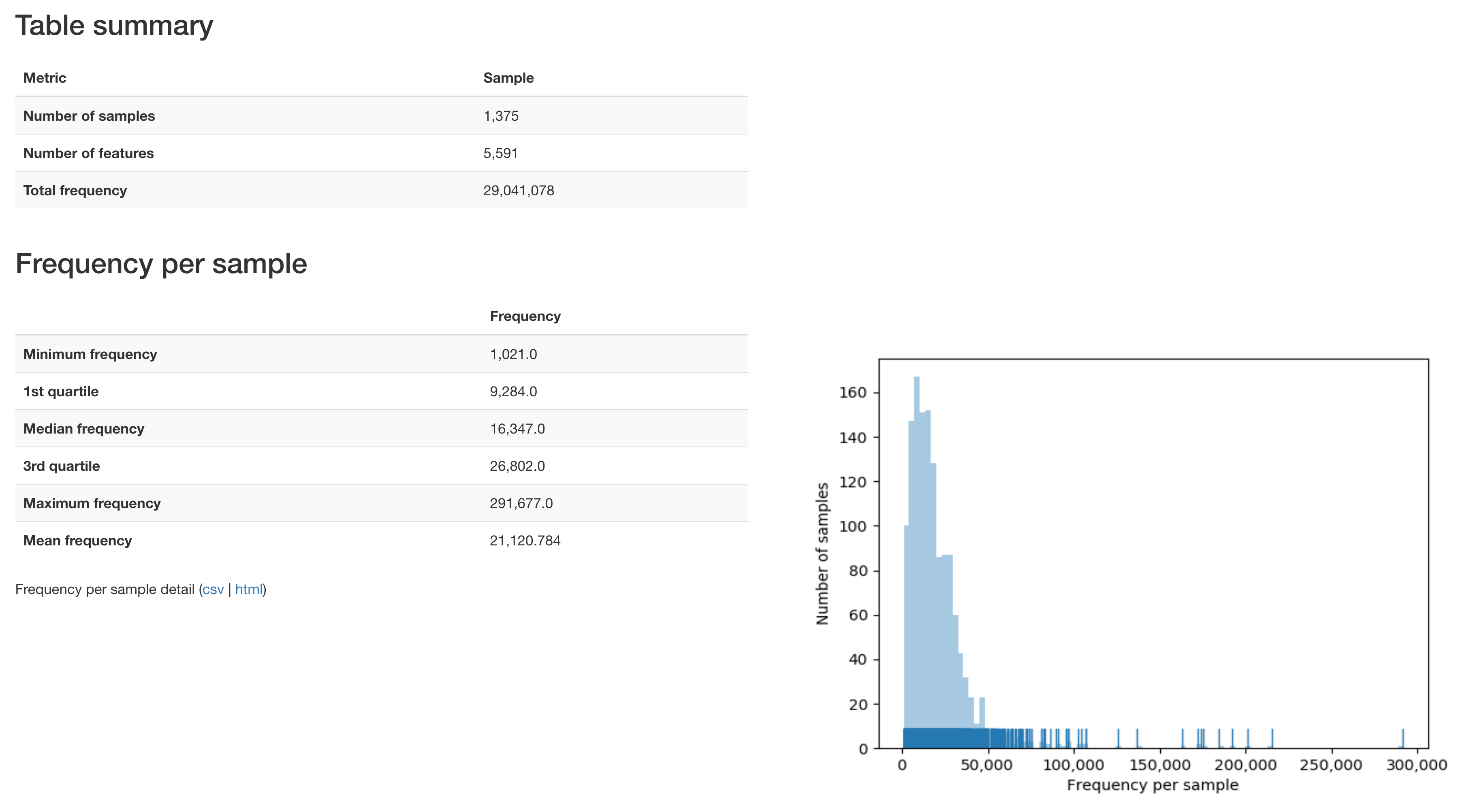
Over 29 million sequences passed QC and were assigned to samples.

Quality Control

What should we do to improve the resolution and remove noise?

1. Filter features from the observation table by:

• Minimum or maximum frequency (counts across samples)
• Minimum or maximum ubiquity (proportion of samples)
• Where metadata is equal to a certain value
• Removing specific samples by the unqiue id

Options for specifically filtering features:

• Lots of options: qiime feature-table filter-features –help

--i-table ARTIFACT_PATH
	The feature table from which features should be filtered. [required]
--p-min-frequency INTEGER
	The minimum total frequency that a feature must have to be retained. [default: 0]
--p-max-frequency INTEGER
	The maximum total frequency that a feature can have to be retained. If no value is provided this will default to infinity (i.e., no maximum frequency filter will be applied). [optional]
--p-min-samples INTEGER
	The minimum number of samples that a feature must be observed in to be retained. [default: 0]
--p-max-samples INTEGER
	The maximum number of samples that a feature can be observed in to be retained. If no value is provided this will default to infinity (i.e., no maximum sample filter will be applied). [optional]
--m-metadata-file MULTIPLE_PATH
	Metadata file or artifact viewable as metadata. This option may be supplied multiple times to merge metadata. Feature metadata used with where parameter when selecting features to retain, or with exclude_ids when selecting features to discard. [optional]
--p-where TEXT	SQLite WHERE clause specifying feature metadata criteria that must be met to be included in the filtered feature table. If not provided, all features in metadata that are also in the feature table will be retained. [optional]
--p-exclude-ids
	Samples to remove
--p-no-exclude-ids
	If true, the features selected by metadata or where parameters will be excluded from the filtered table instead of being retained. [default: False]
--o-filtered-table ARTIFACT_PATH
	FeatureTable[Frequency] The resulting feature table filtered by feature. [required if not passing –output-dir]
--output-dir DIRECTORY
	Output unspecified results to a directory

Let’s remove really rare features, to cut down on sequencing artefacts

• This is filtering by total abundance

Let’s also remove features not in at least 20% of samples

• The percentage or proportion of individuals a feature appears in is known as the ubiquity

# Filter features with less than 50 total counts across all samples
qiime feature-table filter-features \
   --i-table american_gut/1_1_biom.qza \
   --o-filtered-table american_gut/1_2_biom_min_50.qza \
   --p-min-frequency 50

# Filter features in less than 20 percent of samples
# Note: I know N = 1,375 / 5 = 275
qiime feature-table filter-features \
   --i-table american_gut/1_2_biom_min_50.qza \
   --o-filtered-table american_gut/1_2_biom_min_50_ubiq_20.qza \
   --p-min-samples 275

# Summarize the table
qiime feature-table summarize \
   --i-table american_gut/1_2_biom_min_50_ubiq_20.qza \
   --o-visualization american_gut/1_2_biom_summary.qzv

# View the table summary
qiime tools view american_gut/1_2_biom_summary.qzv

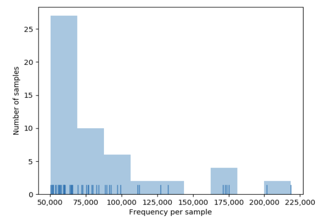
Let’s see how we did:

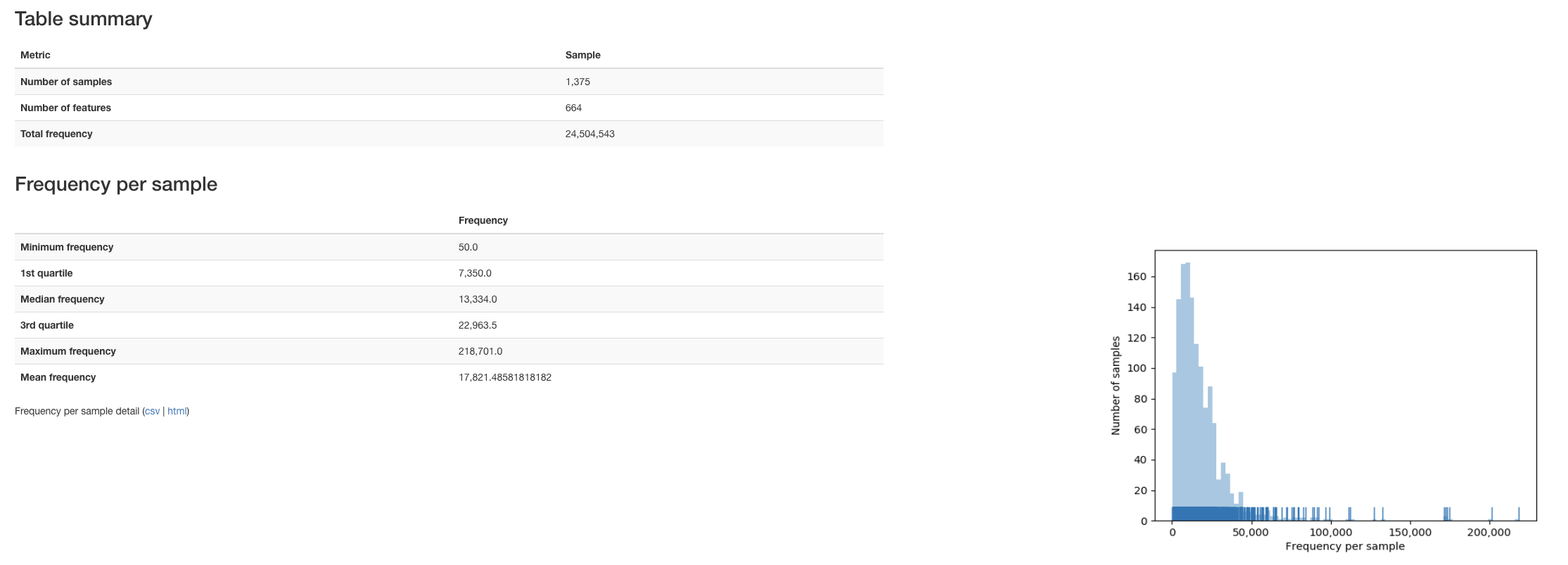
Looks like we cut down our features from 5,590 to 664, not bad…

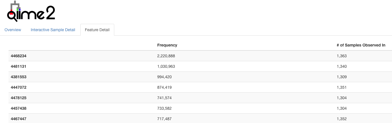
A few features dominate the counts…

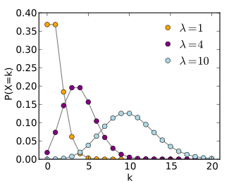
Keep in mind that microbiome counts are not normally distributed

• More often follow a Poisson / Negative Binomial distribution
• This roughly means there are often many low / rare values and some very high outliers

Different Poisson distributions can be modeled, microbiome counts will look like the yellow most often. Source: Wikipedia

We also want to remove samples with low counts, and there is a nice tool to choose that cutoff…

Keep in mind you could also:

• Remove particular microbial taxon: –p-exclude Wolbachia
• Remove specific samples: –p-exclude-ids samples-to-remove.tsv
• Remove samples based on metadata: –p-where “sex IN (‘male’, ‘female’)”

2. We can remove samples with the filter-samples tool

Let’s remove samples with less than 50,000 counts

• This is a high cutoff, and will cut us down to only 53 samples
• This will make the tutorial easier, but 1,000 or 10,000 is often more than adequate

qiime feature-table filter-samples \
   --i-table american_gut/1_2_biom_min_50_ubiq_20.qza \
   --o-filtered-table american_gut/1_3_biom_samplemin_50k.qza \
   --p-min-frequency 50000

qiime feature-table summarize \
   --i-table american_gut/1_3_biom_samplemin_50k.qza \
   --o-visualization american_gut/1_3_biom_summary.qzv

qiime tools view american_gut/1_3_biom_summary.qzv

This is nice for our purposes today, but note that some samples still have much higher counts than others…

Let’s work with this cleaner data, while keeping in mind there are tons of other ways to filter!

• Remove sequences before Deblur feature analysis: qiime quality-control exclude-seqs
• Remove samples and features based on the mock community: qiime quality-control evaluate-composition
• More extensive filtering documentation.

Keep in mind:

• At this point in a real analysis I would back up the filtered files

Community Transformation and Examination

Let’s look at the data beyond just a table summary!

The feature-table tool has a lot of options:

qiime feature-table --help

Commands:

-core-features	Identify core features in table
-filter-features
	Filter features from table
-filter-samples
	Filter samples from table
-filter-seqs	Filter features from sequences
-group	Group samples or features by a metadata column
-heatmap	Generate a heatmap representation of a feature table
-merge	Combine multiple tables
-merge-seqs	Combine collections of feature sequences
-merge-taxa	Combine collections of feature taxonomies
-presence-absence
	Convert to presence/absence
-rarefy	Rarefy table
-relative-frequency
	Convert to relative frequencies
-subsample	Subsample table
-summarize	Summarize table
-tabulate-seqs	View sequence associated with each feature

Options include:

• filtering
• grouping / collapsing
• transforming - rarefy, relative abundance, presence / absence
• creating summaries and figures

I’d suggest creating shortcut variables for the data we imported:

• It’s easier than typing the full path everytime, and easier to remember
• Their names can be arbitrary, I like to go with something logical though

• For best practices they should be called with quotes and a number sign

  • “$XXXXX”
  • Without the number sign it will be treated as a word and not a variable holding something else
  • The quotes are optional today, but in more complex work they will save you a lot of weird errors

• If you wanted to analyze different data you only have to switch paths in one place, not in every function call

# The Feature table can now be called as: "$table"
table=american_gut/1_3_biom_samplemin_50k.qza
echo "$table"
echo $table
echo table

# The taxononomy table can now be called as: "$tax"
tax=american_gut/1_1_tax.qza
echo "$tax"

# The phylogeny can now be called as: "$tre"
tre=american_gut/1_1_tree.qza
echo "$tre"

# The metadata can now be called as: "$map"
map=american_gut/1_0_map.txt
echo "$map"

So let’s exmaine how our community is taxonomically distributed!

• Barplots of the taxonomic distribution of features for each sample
• These plots are based on relative abundance within a total sample
• Do not provide information about absolute microbial load

• Note below how I use the shortcuts instead of writing out full paths…

  • It just looks so much cleaner too!

# Make and view a taxonomy barplot
qiime taxa barplot \
   --i-table "$table" \
   --i-taxonomy "$tax" \
   --m-metadata-file "$map" \
   --o-visualization american_gut/2_0_taxonomy_barplot.qzv

qiime tools view american_gut/2_0_taxonomy_barplot.qzv

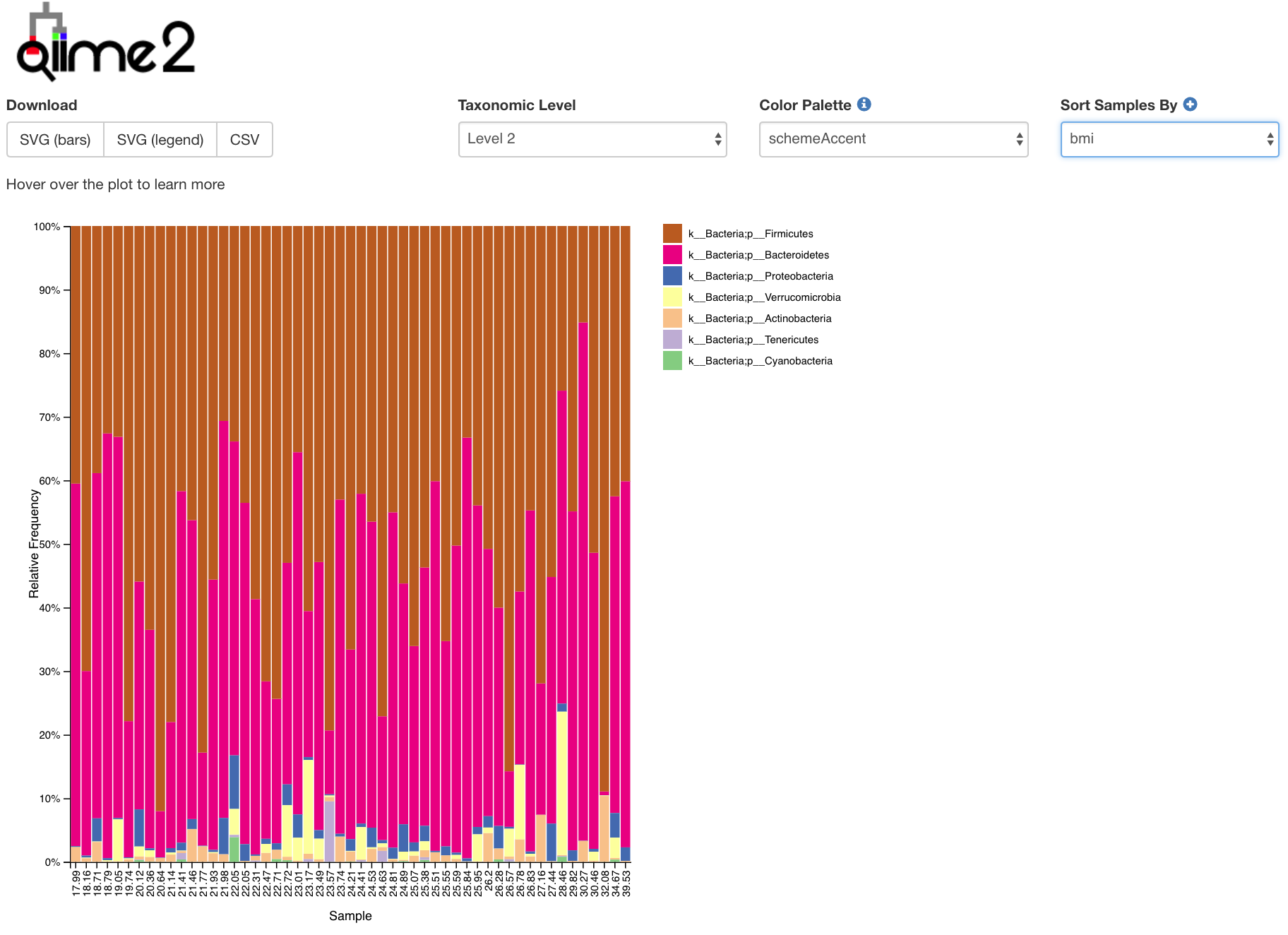
This is a really useful tool for examining our microbial communities

• Just remember how the relative abundance works…

  • Everything is relative to everything else!
  • One abundant microbe decreasing makes rarer microbes look more abundant
  • One abundant microbe increasing makes rarer microbes look less abundant

Rarefaction and Normalization

Raw counts are biased:

• Samples have different numbers of sequence counts
• Not indicative of absolute bacterial abundance
• Artifact of extraction, library preparation and pooling, and sequencing efficiency

Some ways to transform the counts:

-presence-absence
	Convert to presence/absence
-rarefy	Rarefy table
-relative-frequency
	Convert to relative frequencies

qiime feature-table presence-absence \ ...
qiime feature-table rarefy \ ...
qiime feature-table relative-frequency \ ...

Presence / Absence: value of 1 if taxon is present in sample, 0 otherwise

Rarefy: subsample the same number of sequence from each sample

Relative Frequency: propotion of each feature out of the total feature counts for each sample

There are other normalization methods, often based on RNA sequencing methods.

• Generally seem more biased than rarefy / relative abundance
• Better fit in standard sense, don’t seem to adapt well to wide bias across different datasets

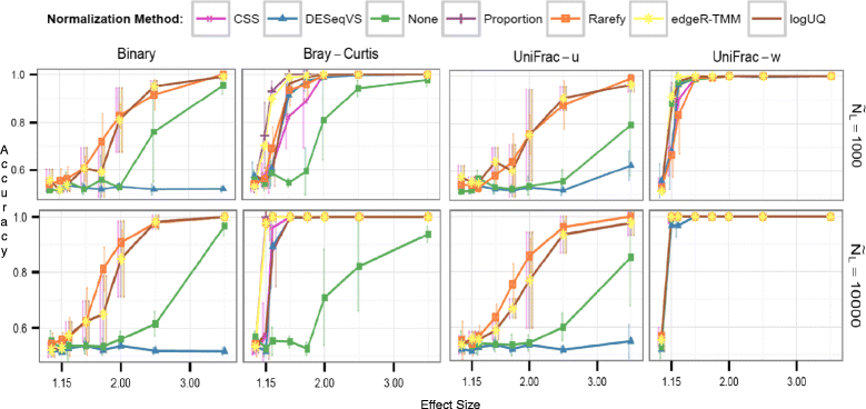
Comparison of different methods to control for different sequence counts. Purple and Orange are what we care about! Source: Weiss, S. et. al. Microbiome. 2017

-None	No correction for unequal library sizes is applied
-Proportion	Counts in each column are scaled by the column’s sum
-Rarefy	Each column is subsampled to even depth without replacement (hypergeometric model)
-logUQ	Log upper quartile—Each sample is scaled by the 75th percentile of its count distribution; then, the counts are log transformed
-CSS	Cumulative sum scaling—This method is similar to logUQ, except that CSS enables a flexible sample distribution-dependent threshold for determining each sample’s quantile divisor. Only the segment of each sample’s count distribution that is relatively invariant across samples is scaled by CSS. This attempts to mitigate the influence of larger count values in the same matrix column
-DESeqVS	Variance stabilization (VS)—For each column, a scaling factor for each OTU is calculated as that OTU’s value divided by its geometric mean across all samples. All of the reads for each column are then divided by the median of the scaling factors for that column. The median is chosen to prevent OTUs with large count values from having undue influence on the values of other OTUs. Then, using the scaled counts for all the OTUs and assuming a Negative Binomial (NB) distribution, a mean-variance relation is fit. This adjusts the matrix counts using a log-like transformation in the NB generalized linear model (GLM) such that the variance in an OTU’s counts across samples is approximately independent of its mean
-edgeR-TMM	Trimmed Mean by M-Values (TMM)—The TMM scaling factor is calculated as the weighted mean of log-ratios between each pair of samples, after excluding the highest count OTUs and OTUs with the largest log-fold change. This minimizes the log-fold change between samples for most OTUs. The TMM scaling factors are usually around 1, since TMM normalization, like DESeqVS, assumes that the majority of OTUs are not differentially abundant. The normalization factors for each sample are the product of the TMM scaling factor and the original library size

Summary: I’d suggest sticking to relative abundance and rarefied communities!

• Remember how many things can bias microbiome data
• The Poisson / Negative Binomial fit in more advanced models doesn’t seem to adapt well

Alpha and Beta Diversity

We can use ecological metrics to understand community composition and inter-sample microbiome similarity!

Alpha Diversity: Measure of diversity within a sample

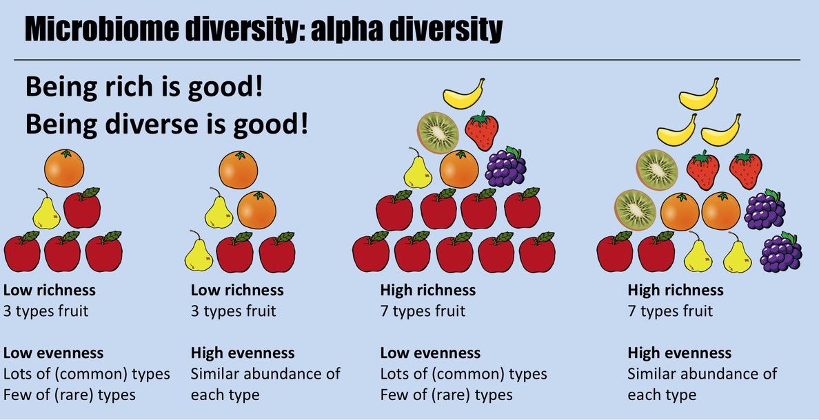
Alpha diversity metrics can look at richness, evenness, or both within a sample. Source: Finotello. Briefings Bioinformatics. 2016.

Beta Diversity: Measure of microbiome similarity between a pair of samples

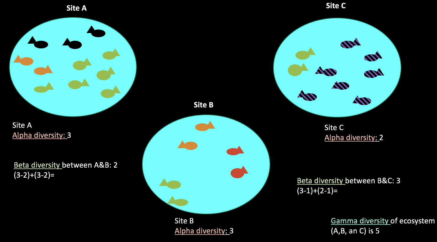
Beta diversity calculates how similar two total ecosystems are. Source: Kate M. Socratic.org.

There are many metrics (ways to measure) Alpha and Beta Diversity

Both Alpha and Beta Diversity can take into account the microbial phylogeny with certain metrics

Metrics are assigned with the -p-metric argument:

# Alpha Diversity - Non-Phylogenetic Observed OTUs
qiime diversity alpha \
  --i-table "$table" \
  --p-metric observed_otus \
  --o-alpha-diversity american_gut/2_2_observed_otus_vector.qza

# Alpha Diversity - Non-Phylogenetic Observed OTUs
qiime diversity alpha-phylogenetic \
  --i-table "$table" \
  --i-phylogeny "$tre" \
  --p-metric faith_pd \
  --o-alpha-diversity american_gut/2_2_faith_pd_vector.qza

# Beta Diversity - Non-Phylogenetic Bray-Curtis
qiime diversity beta \
  --i-table "$table" \
  --p-metric braycurtis \
  --o-distance-matrix american_gut/2_2_unweighted_unifrac_distance_matrix.qza

# Beta Diversity - Phylogenetic Unweighted UNIFRAC
qiime diversity beta-phylogenetic \
   --i-table "$table"\
   --i-phylogeny "$tre" \
   --p-metric unweighted_unifrac \
   --o-distance-matrix american_gut/2_2_unweighted_unifrac_distance_matrix.qza

QIIME2 has done a good job wrapping diversity computation with my favorite metrics into one easy script:

• Rarefies the table to a specified depth (necessary for diversity to be computed accurately)

• Calculates Alpha and Beta Diversity

  • Alpha Metrics:

    • Faith’s PD: Phylogenetic diversity
    • Observed OTUs: Richness of community
    • Shannon: Balances richness and evenness
    • Pielou’s Evenness: Evenness of community

  • Beta Diversity

    • Unweighted Unifrac: Presence / absence phylogenetic distance between samples
    • Weighted Unifrac: Abundance weighted phylogenetic distance between samples
    • Jaccard: Presence / absence distance between samples
    • Bray Curtis: Abundance weighted distance between samples

• Can be parallelized across multiple CPUs
• Generates output visuals

Options:

--i-table ARTIFACT_PATH
	The feature table containing the samples over which diversity metrics should be computed. [required]
--i-phylogeny ARTIFACT_PATH
	Phylogenetic tree containing tip identifiers that correspond to the feature identifiers in the table. This tree can contain tip ids that are not present in the table, but all feature ids in the table must be present in this tree. [required]
--p-sampling-depth INTEGER_RANGE
	The total frequency that each sample should be rarefied to prior to computing diversity metrics. [required]
--m-metadata-file MULTIPLE_PATH
	Metadata file or artifact viewable as metadata. This option may be supplied multiple times to merge metadata. The sample metadata to use in the emperor plots. [required]
--p-n-jobs INTEGER_RANGE
	The number of jobs to use for the computation. This works by breaking down the pairwise matrix into n_jobs even slices and computing them in parallel. If -1 all CPUs are used. If 1 is given, no parallel computing code is used at all, which is useful for debugging. For n_jobs below -1, (n_cpus + 1 + n_jobs) are used. Thus for n_jobs = -2, all CPUs but one are used. (Description from sklearn.metrics.pairwise_distances) [default: 1]

Let’s get it running, then I can explain it…

qiime diversity core-metrics-phylogenetic \
   --i-phylogeny "$tre" \
   --i-table "$table" \
   --p-sampling-depth 50000 \
   --m-metadata-file "$map" \
   --output-dir american_gut/2_3_diversity_core_phylogenetic

Note the –p-sampling-depth Option:

• This is the depth we will rarefy for each sample
• Since we know each sample has 50,000 counts we will use that
• Essentially we are just randomly picking 50,000 counts from each sample
• While effect size matters, rarefy depth doesn’t hugely affect ability to detect a signal
• More samples is stronger than deeper rarefy depth! Don’t throw away info

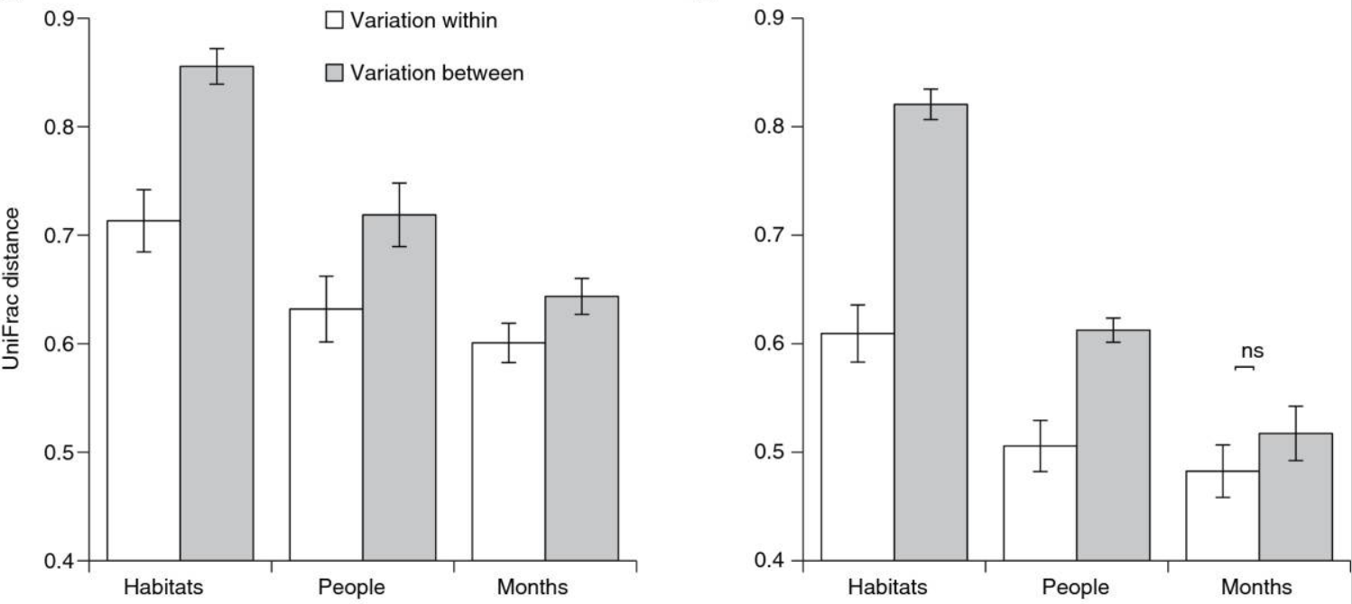
The left figure is rarefied to 1,500 seqs/sample, the right is rarefied to 10 seqs/samples. Source: Kuczynski, J. Genome Biology. 2010

# List files in diversity results
ls -lsh american_gut/2_3_diversity_core_phylogenetic/

What do you notice about the types of files that were made?

If for some reason you don’t have a phylogeny, there is a non-phylogenetic wrapper method

• One could also aruge about the degree to which functional similarity parallels genetic similarity of the 16S rRNA gene

Let’s look at the alpha diversity

• Here I get a bit more fancy, wrapping each of the metrics in a for loop
• Don’t have to write the ‘qiime diversity alpha-group-significance…’ command four times

# Create a shortcut to our diversity output folder
diversity_folder=american_gut/2_3_diversity_core_phylogenetic/

##### ALPHA DIVERSITY ANALYSES #####
# for each alpha diversity metric...
for alpha_metric in faith_pd shannon observed_otus evenness
do
   # print the diversity vector name
   echo "$diversity_folder""$alpha_metric"_vector.qza

   ### ALPHA ASSOCIATION CATEGORICAL MAPPING ###
   qiime diversity alpha-group-significance \
      --i-alpha-diversity "$diversity_folder""$alpha_metric"_vector.qza \
      --m-metadata-file "$map" \
      --o-visualization american_gut/2_4_"$alpha_metric"_group_significance.qzv

# Close the for loop
done

Using a for loop and shortcut to the diversity folder are really nice because

• We could easily add or remove alpha metrics
• We could apply this to a different diversity folder by changing one line
• Think about making you code flexible when building pipelines!!!

# Variable you can change to easily see other metrics
alpha_metric=shannon

# View Alpha diversity results
qiime tools view american_gut/2_4_"$alpha_metric"_group_significance.qzv

Take note of the statistics included

• Which groups have
• Keep in mind corrections for multiple variables

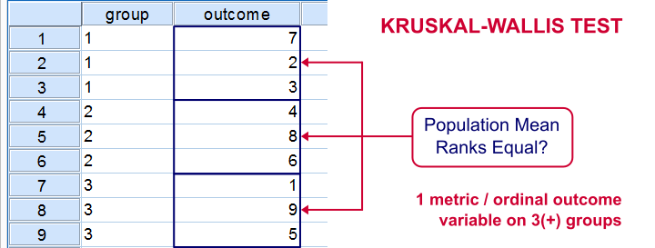
Kruskal Wallis is non-parametric because it uses the rank order and not the actual values. Source: spss-tutorials.com

Let’s look at the beta diversity

• Here is another useful trick for running different metrics, commenting them out
• Note that if two are left active the beta_metric will be set to the last call

# Variable you can comment on / off to easily see other metrics, only use one at a time
beta_metric=weighted_unifrac
#beta_metric=unweighted_unifrac
beta_metric=bray_curtis
#beta_metric=jaccard


# View Alpha diversity results
qiime tools view "$diversity_folder""$beta_metric"_emperor.qzv

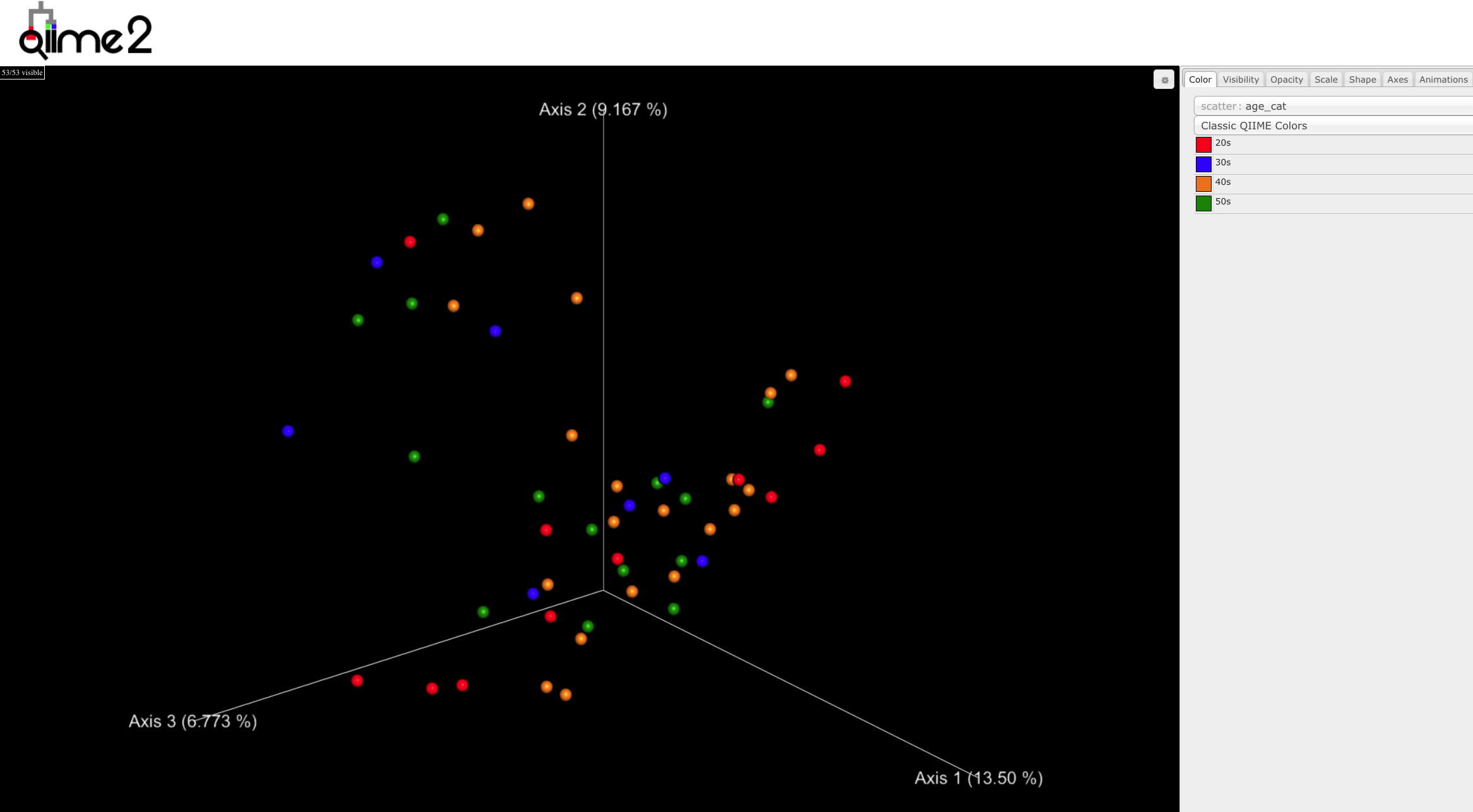
Principle Coordinates of Analysis (PCoA)

We will talk about this in more detail, and specific ways to test hypotheses. Click ‘Next’ down to the right